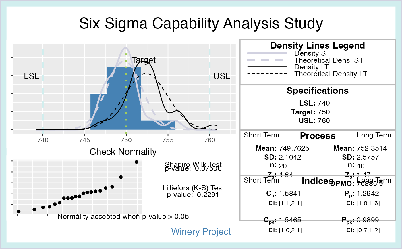
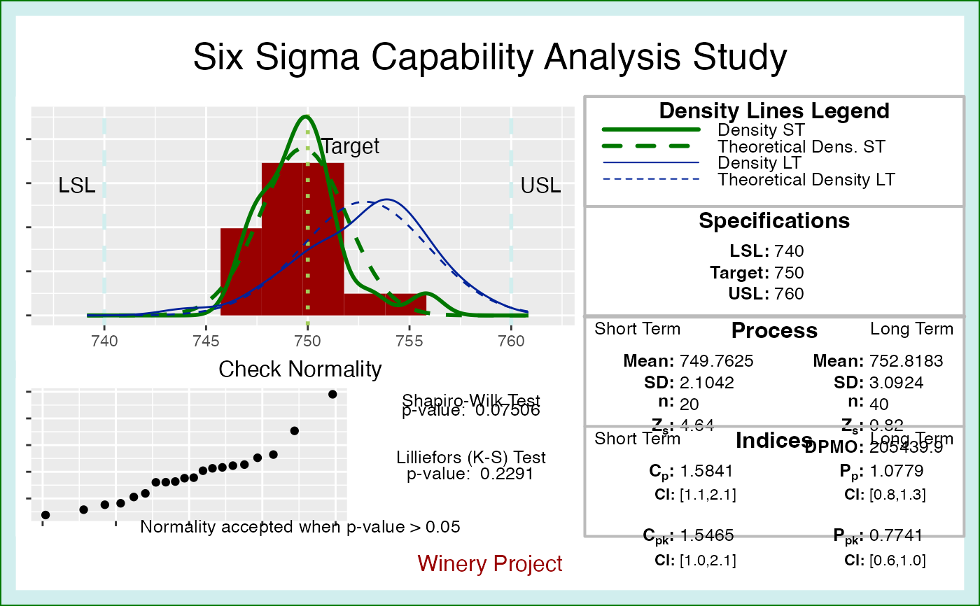
Plots a Histogram with density lines about the data of a process. Check normality with qqplot and normality tests. Shows the Specification Limits and the Capability Indices.
ss.study.ca(
  xST,
  xLT = NA,
  LSL = NA,
  USL = NA,
  Target = NA,
  alpha = 0.05,
  f.na.rm = TRUE,
  f.main = "Six Sigma Capability Analysis Study",
  f.sub = "",
  f.colours = c("#4682B4", "#d1d1e0", "#000000", "#A2CD5A", "#D1EEEE", "#FFFFFF",
    "#000000", "#000000")
)
Arguments
- xST
Short Term process performance data
- xLT
Long Term process performance data
- LSL
Lower Specification Limit of the process
- USL
Upper Specification Limit of the process
- Target
Target of the process
- alpha
Type I error for the Confidence Interval
- f.na.rm
If TRUE NA data will be removed
- f.main
Main Title for the graphic output
- f.sub
Subtitle for the graphic output
- f.colours
Vector of colours fot the graphic output
Value
Figures and plot for Capability Analysis
Note
The argument f.colours takes a vector of colours for the graphical outputs. The order of
the elements are, first the colour for histogram bars, then Density ST lines, Density LT
lines, Target, and Specification limits. It can be partially specified.
References
Cano, Emilio L., Moguerza, Javier M. and Redchuk, Andres. 2012. Six Sigma with R. Statistical Engineering for Process Improvement, Use R!, vol. 36. Springer, New York. https://link.springer.com/book/10.1007/978-1-4614-3652-2/.
Montgomery, DC (2008) Introduction to Statistical Quality Control (Sixth Edition). New York: Wiley&Sons

